Artificial Intelligence integrated framework for stability of functions in persistent homology
Allan Onyango1, Benard Okelo1, Priscah Omoke1
1Department of Pure and Applied Mathematics, Jaramogi Oginga Odinga University of Science and Technology,
P. O. Box 210-40601, Bondo, Kenya.
Corresponding Author:Benard Okelo (e-mail: bnyaare@yahoo.com)
DOI: https://doi.org/10.59461/ijdiic.v4i2.195
Article history: Received March 26, 2025, Revised May 24, 2025, Accepted June 15, 2025
ABSTRACT
Explaining the spatial properties in point set topological spaces is a tough task. Experts in TDA have sought to discover if it is possible to find a strong intuition about the geometry and topology in big datasets, easily seen when dealing with all of them at the same time. This point also notes that the estimates will stay useful if we can detect whether the constants remain stable as the data changes, for instance, the Hausdorff distance function when the data exhibits noise, or even when a little noise is added to the point-cloud datapoints. This could happen if these properties are considered in topologically invariant compact subsets of X, which requires very stringent and restrictive assumptions to obtain well-defined shapes that can be drawn from the data in the compact subsets. The aim of this study is to outline factors that make functions in persistent homology stable. The results show that factors like triangularability affect stability of functions. Moreover, we have given an integrated artificial intelligence (AI) framework for stability of functions, to trace the accuracy levels of algorithms in cyber-threat identification and cyber-threat attacks using Persistent Homology.
This is an open access article under the CC BY-SA license.

Keywords: Artificial intelligence, Persitent homology, Integrated Framework, Stability
1. INTRODUCTION
Topological Data Analysis (TDA) comprises a new mathematical domain, which involves techniques and tools that exploit topological information obtained from the ”shape” of data. These tools continue to prove instrumental in extracting important, globally high-dimensional features from datasets that have proven challenging to analyze using traditional analysis techniques.
Topology, as defined in the influential work Analysis Situs by [1], refers to the mathematical examination of structures that remain unchanged under continuous deformation. It is a formalized field that focuses on the geometry of position. For more than a century, the concept of shape was only studied in the field of pure mathematics. Nevertheless, the emergence of persistent extracts, which enable scientists to compute compact visualizations of the topological data with robust conceptual guarantees, has resulted in the utilization of TDA and ML shapes. Topology is a mathematical discipline that focuses on studying shapes. It involves characterizing spaces based on their structure, which remains unchanged even when the space is continuously deformed. Leibniz referred to this as Analysis Situs, which can be understood as the study of the spatial arrangement of objects. In his influential paper titled ”On the Foundations of Geometry,” he defined it as the skill of effectively reasoning based on poorly drawn figures. However, for these figures to be reliable, they must meet specific criteria. While the proportions can be significantly distorted, the relative positions of the various components must remain unchanged.
In a subsequent section of the study, the author provided a formal definition of homeomorphism [2]. This function has the ability to alter and elongate the space in which it is applied. In other words, the fundamental structure of the space remains unchanged. A doughnut and a mug can be topologically identical since they are homeomorphic, that is, they can be continuously and bijectively deformed into one another. This is the classic illustration of homeomorphism.

Figure 1. Broken topological configuration
Figure 1 illustrates homeomorphisms, displaying an artistic representation of these continuous deformations. To get a deeper comprehension of systems with the same topology, mathematicians sought to identify topological invariants: characteristics of spaces that remain constant regardless of homeomorphism. Dimensionality is a topological invariant, as demonstrated by [3]. Not too long after [4] proposed the Betti number to investigate the p-dimensional connectedness of spaces, [5] demonstrated that it was a topological invariant. Colloquially, the Betti number β0 represents the quantity of linked elements, β1 represents the quantity of cavities, and β2 represents the quantity of empty spaces.
The best way to think of Betti numbers could simply be as an algebraic group Hp that encodes some topological structure, or homology groups, as an invariant of those groups. It is determined by topological invariants that two homeomorphic spaces have isomorphic homology groups. An isomorphism is a function f that takes G and H to each other, is bijective, and meets the property that f(gh) = f(g)f(h). For an equivalence class with a set topological feature, the homological group and the rank of Hp, we use the Betti number βp for short. According to [6], a topologist and codebreaker at Bletchley Park, [7]’s work provided a comprehensive understanding initially of the topological invariants’ mathematical importance.
More than a hundred years after Poincaré’s work on Analysis Situs, topologists presented a strong argument for using topological techniques in TDA. One such work was [8] ”Topology and Data,” where he proposed that high-dimensional noisy datasets might be effectively represented by theoretically grounded topological summaries. Persistent homology is one of the methods he talks about. Persistence arose from investigations into both size functions and topology in dynamical systems and involves calculating homology across a filter consisting of carefully chosen spaces. Usually, to determine persistent homology groups, a filtration is formed by using several linked simplicial complexes. An abstract simplicial complex is something like a graph, where each p-dimension △ inside it is called a simplex. A zero-simplex is just a singular vertex, but with p-simplexes (p > 0), you have p + 1 vertices [9].
Persistent Betti number βi,j, derived from the filtering {Ki}i∈I, quantifies the count of p-dimensional homological components existing in Ki while it continues its existence in Kj. This offers the initial algorithm for efficiently calculating the βi,j while introducing the Persistence Barcode (PB) as a way to encode the PH. The aforementioned illustrates the emergence and demise of the homology classifications, that is, these locations within these filter {Ki}i∈I where a PH classification starts from Ki as it disappears (turns into zero) at Kj. It should be noted that the set Kϵ ⊆ Kϵ′ whenever the value of ϵ is less than or equal to the value of ϵ′. In this scenario, ϵ is a threshold that is used to determine the maximum allowable Euclidean distance between points.

Figure 2. A process of separating simplicial complexes based on specific criteria
Figure 2: Once the theoretical underpinnings were established, the area of Topological Data Analysis (TDA) was ready to flourish. First, PD and associated feature indicators were studied through the creation of data on the persistence diagram space. Nevertheless, PD is neither an optimal portrayal for use with subsequent techniques for analyzing data due to its costly computation of distances, nor lack of unique means, and dependence on the underlying data’s topology for numerical datapoints. Consequently, numerous feature extraction algorithms were suggested to mirror PDs on a vector in Rn. However, we concur with [10] that due to the persistence diagram’s extensive invariance, any plausible method of representing it as a vector tends to yield satisfactory results.

Figure 3. The persistence diagram and barcode
Figure 3 provides an illustration of this. Once PH was classified as a graded module, it was possible to decompose the Persistence Module (PM) that rightly correlated to the birth-time death-time denominates of the PH classes by applying the structure theorem for finitely generated modules. Building on this concept, which demonstrated its stability as a reliable illustration of operational filters, demonstrated that this representation is an isometry. This PD, a planar illustration of PH, has emerged as the dominant visual description of persistent homology. It is identical to PB, with birth times plotted on the x-coordinate and death times on the y-coordinate. A specific instance is illustrated in Figure 4. This is an instance of a persistence-related condensation, which refers to data illustrations that form the foundation of this work.
Every one of these vectorizations of the PD is likewise a summary based on persistence; we are especially interested in their machine-learning applications in this text. ML is an AI discipline that focuses on the innovations of computing algorithms that have the ability to obtain insights from datasets. This creation of a feature vector that effectively represents the structure of a data set, having reliable conceptual assurances, makes this an ideal choice for utilization in ML approaches.
ML techniques can be classified as either supervised or unsupervised. Supervised algorithms learn a function, denoted fω, having denominations ω, that takes a dataset X to a quantity y using a simulation data set that contains absolute elements. Non-supervised algorithms learn a filtration function f, referring to elements within a data set X that lack precision. Usually, ML algorithms are utilized for either classification or regression tasks. In classification, the goal is to assign input data x ∈ X to a specific category. In regression, the purpose is to take the input dataset x in X and convert it into continuous attributes. We may employ random forests in this work. This is a supervised learning technique that combines the predictions of individual decision trees to be utilized for regression or classification.
Figure 4 displays a Random Forest (RF) consisting of three decision trees. During the training process, every point within a decision tree acquires a parameter and an approach that it subsequently utilizes to generate predictions. For classification tasks, individual predictions are usually combined through majority voting, while for regression tasks, the mean prediction is computed. While a single tree is susceptible to overfitting, an RF greatly enhances performance compared to a single tree, albeit at the expense of reduced interpretability of its predictions [11]. When utilizing persistence-based summaries, we commonly employ random forests as our subsequent models. Additionally, the unsupervised learning process is expanded to incorporate persistence diagrams.
Random forest techniques are occasionally called shallow learning since they learn a relatively small number of parameters. The authors in [12] have spearheaded ground-breaking research that has sparked a profound transformation in deep learning. This revolution has witnessed the remarkable success of models with an extensive number of parameters, often reaching hundreds of billions, across a wide range of tasks. Deep learning models now incorporate topological tools, enabling the learner to get insights into the data’s topology. DL approaches commonly employ gradient descent optimizers, which depend on a loss function L(y, y′) to calculate the discrepancy between the actual labels y and the latest predictions y′ made by the model. By evaluating the discrepancy between the function fω mapping X to y and the actual output, DL could modify the variables ω to minimize the model’s errors. While it has been considered an oversimplification, it implies that if we are able to distinguish this calculation of PDs, it is possible to incorporate topology assumptions to train DL models by including a topology component in the loss function L.
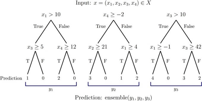
Figure 4. Three decision trees are denoted by a random forest
In this text, we’ll discuss many ways in which the concept of persistence may be applied to solve machine learning challenges. The main concept involves utilizing PDs as Feature Vectors (FV) for input into subsequent ML algorithms. However, various challenges associated with this approach exist. This space of persistence diagrams has significant pathological characteristics. An initial method for navigating this issue involves utilizing persistence landscapes [13]. This process maps PDs onto a Hilbert space, enabling them to be imputed into common ML techniques. Subsequent to that, rank functions and multiple kernels have been developed. In more recent times, there has been research focused on utilizing deep learning to discover optimum functions of persistence diagrams.
Extensive research has been conducted on the statistical characteristics of persistence diagrams and landscapes, which includes the utilization of bootstrapping techniques. These strategies have been utilized in several domains. The most comprehensive use is in the field of geometry processing. By including local characteristics such as curvature or features derived from heat kernels, several geometric structures may be recovered, including symmetry, segmentation, form classification, and retrieval [14].
Persistence diagrams have been shown to be instructive in several applications, including biology. Specifically, they have been found useful in protein docking and simulating circuits in the brain. The last field of application we discuss is material science. Machine learning has not been widely utilized in this particular domain. Partly because the input is noticeably different in nature compared to what is usually encountered in machine learning. Conventional image processing approaches are not effective in handling scientific pictures, such as electron microscope images. The use of topological summaries effectively captures the pertinent structure. This region is now in its first phase, with several other captivating advancements anticipated.
Therefore, it is important to note that PDs may not be the sole topology properties utilized. We note that the Euler Curve had been initially utilized in the analysis of fMRIs [15]. This characteristic has been thoroughly examined in the statistical literature. However, it is demonstrably less useful than persistence diagrams, while being much easier to compute. Furthermore, fMRI has been utilized in several categorization tasks.
Furthermore, outside of offering a valuable synopsis and functionalities for machine learning algorithms, another area of focus is the correlation between the results and the original data. Solving this inverse problem is highly challenging and frequently unattainable in most cases. However, this trend has frequently failed to be as bleak as it may appear. Initial efforts in the field are reevaluating Single Linkage Clustering (SLC) using the concept of persistence [16]. Although it is widely recognized that SLCs are prone to instability, it is feasible to utilize persistence to demonstrate the presence of stable components within the clusters. By employing a ”soft” clustering algorithm, it becomes possible to stabilize the clusters by assigning each data point a probability of being assigned to a particular cluster. Current research aims to identify comparable steady illustrations within datasets from high-dimensional constructions, like cycles.
Another arising issue has been parameterization. To clarify, its goal is to identify inherent coordinates that describe the data by building upon effective methods used in reducing dimensionality. These approaches encompass both linear techniques like PCA and MDS, as well as non-linear techniques like ISOMAP and LLE. The initial study organized texture space by utilizing a Klein bottle as its fundamental structure[17], which had been discovered a few years earlier. However, this was constructed manually. The initial category of generic approaches is the mapping of circular coordinates to data. This is especially advantageous for addressing the issue of recurrence in systems that change over time. Recurrence, which includes periodicity, may be accurately represented using an angle. By combining persistence with least-squares optimization, a systematic method is established for determining these coordinates automatically. This technique was utilized to analyze and describe human movements, including various types of walking and other physical actions. Subsequent research has demonstrated the method of creating coordinate systems for objects with more dimensions using the projective plane.
One further approach we contemplate is incorporating topological restrictions into machine learning algorithms. In this study, topology priors were employed to assist with the process of selecting the variable. For instance, the refurbishment of a racecourse could consist of a single component and one gap, which becomes its major foundation [18]. By calculating the persistence with regard to a regeneration variable, such as the bandwidth of a kernel, we may determine the optimum variables resulting in the desired topological structure of the reconstruction. The encoding of topological constraints is now in its nascent phase, although it holds the prospective to offer a novel kind of regularization to ML algorithms.
Let us, at this point, consider a standard TDA pipeline (Figure 5). The input variable consists of a collection of samplings, which are typically, but not necessarily, contained within a metric space. The underlying space of data is represented multiscalely, considering the metric as well as other functions (like density). This extends the analysis beyond considering only relationships between pairs of items to incorporate information on relationships between several items. Subsequently, persistent homology is utilized. This tool is derived from algebraic topology and provides a concise representation of the entire multiscale structure representing a PD [19]. Subsequently, the condensed depiction could be utilized in diverse applications.
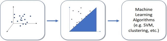
Figure 5. Standard TDA pipeline
The representations of the underlying space are constructed by assembling basic components and connecting them together. There are numerous methodologies for this, but the most straightforward one is arguably the Simplicial Complex (SC). Forming the simplex is achieved by taking a convex combination of k points. A point is a singular entity; we form an edge by combining 2 points, a triangle is created by three points, a tetrahedron is formed by 4 points, and so on (Figure 6). In a broader sense, k-dimensional simplices are defined as the result of combining points of (k + 1) in a convex manner. In a graph, an edge symbolizes a relationship between two entities. Similarly, triangles symbolize interactions involving three entities, whereas higher dimensional simplices represent relationships involving more than three entities. A graph is a one-dimensional complex because it captures all pairwise information while disregarding any higher-order information. By using higher dimensional simplices, we are able to incorporate more detailed information, resulting in more precise templates [20]. It’s worth noting that these designs should not exist in a physical area, but instead reflect information about connectedness. The study of the geometric realization of simplicial complexes in combinatorics has a lengthy historical background, but we will not discuss it in this context. When moving from the left to the right, a vertex is considered to have zero dimensions, an edge has one dimension, a triangle has two dimensions, and a tetrahedron has three dimensions.
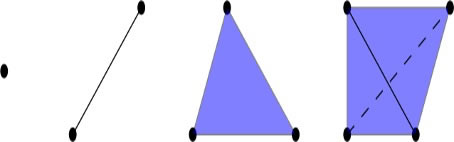
Figure 6. Simplicies dimensions
There exist three primary impediments to this form of modeling. One of the primary issues is the absence of sufficient data. Paradoxically, despite the abundance of big data, we frequently encounter a dearth of data. This is a result of the lack of consistency and uniformity in the data. Considering 10-way associations may be impractical if this data is only accessible for a limited portion of the data. The second aspect is computation. When examining higher-order relationships, there is typically a significant increase in complexity since one needs to analyze all possible combinations of k-tuples. This results in preprocessing demands that are impractical to fulfil. The ultimate challenge lies in the interpretability. Although we can comprehend a simplex on a local scale, comprehending its global structure becomes progressively more difficult.
This serves as the initial reference for the tools we will be discussing later. A significant portion of the machine learning research focused on graphs aims to comprehend the inherent qualitative characteristics of the underlying graph. Statistical properties like degree distributions, centrality measures, and diameter are commonly computed on the network. In order to capture more complex patterns, we need to utilize a distinct set of techniques. Initially, it is important to observe that a group of simplices can be assembled in a cohesive manner. Within graphs, edges could possibly intersect along edges. Similarly, simplices could possibly be connected along lower-dimensional simplices, such as triangles intersecting along edges or at a vertex [21]. This imposes a limitation on the manner in which basic components (such as simplices) can be joined together to create a spatial structure. Although the representation of spaces is not significantly restricted, it does provide us with more organization.
The initial step in the introduction is elucidating the glueing map, which is referred to as the border operator. Each k-simplex is defined by its boundary, which consists of a set of k-1 simplices. For instance, an edge boundary is defined by its two endpoints, while the triangle’s border is defined by its three edges (Figure 7). The representation thereof could be expressed in the form of a matrix, where columns represent k-simplices while rows represent k-1 simplices, denoted as ∂k. We demonstrate here that a triangle has three edges as its border, and an edge has two vertices.
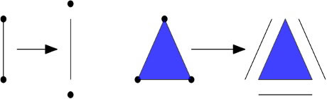
Figure 7. Attachment of every simplex to its border
This kernel refers to the set of k-simplices that constitute the null space of the matrix associated with cycles. Notably, this aligns with the idea behind cycles within graph theory. We completely ignore any cycles that are formed by higher-dimensional simplices within bounded regions. The volume that remains turns into a number of k-voids in the mentioned space. In fact, homology of dimension 0 counts the number of joined elements, and homology of dimension 1 counts the number of holes. The k-th Betti number, βk, measures the total number of different features in a certain object. This is similar to the matrix rank, which represents the count of fundamental elements that a vector space possesses. This provides a subjective depiction of the space.
The success of TDA has been slowed by the challenges encountered while implementing its basic functional tool, the barcode or persistence diagram, in collaboration with machine learning and statistics. More studies need to be done on TDA implementations using the persistence landscape. All science disciplines have experienced massive data generation in recent years; hence, modern society, including scientists, industry, and the public, has been met with a new challenge of obtaining relevant tools to make sense of this Big Data. Normally, features extracted by Topological Data Analysis techniques become perceived as a summary of properties of topology, which define a geometric object as shown in Figure 8.
The goal of TDA is to come up with acceptable techniques to analyze, identify, and utilize the multidimensional properties of geometry and topology [22]. In spite of TDA being on its sunrise days, and rapidly growing, it has already achieved a milestone of fully fledged and coherent tools that are a supplement to other data science techniques, which have made them beneficial to implementations in industrial problems applying TDA algorithms. These algorithms are user-friendly and open source through excellent libraries, which comprise the GUDHI repository, which comprises both Python and C++, as well as R counterparts, Dionysus, PHAT, DIPHA, or Giotto.
As of the last decade, the explosive data generation with gradual complexity has been motivated by the popularity of simulation tools and measurement devices, and this has in return posed more challenges in data analysis: data continually appear as points within high-dimensional spaces, as complex 2-dimensional or 3-dimensional images, an interconnected shapes, a multidimensional time series, or as a graph [23]. These new challenges have been remedied by the recent advances in new relevant mathematical theorems from geometry and topology. As a matter of fact, geometrical and topological patterns instrumental in data analysis have been revealed, which have proved useful for additional machine learning explorations.
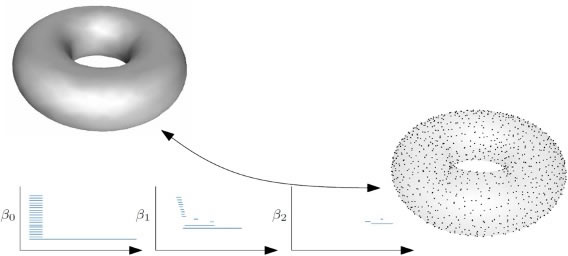
Figure 8. TDA estimate of the underlying object
Courtesy of the principles of stability, persistence diagrams have proven very useful as topological data signatures. In fact, users find it easy to obtain meaning from persistent diagrams because the lifespan of most of the topological features is represented by persistence intervals. This has made persistence diagrams a centre of interest during machine learning and other data analysis processes. The authors in [24] reveal similar classification scenarios and detail industrial implementations towards arrhythmia classification. The stability theorem for persistent homology proves that their study points to TDA’s absolutely powerful principle. The incentive behind it seems obvious: if PH is to be of utmost value, and if two topological spaces X, Y are close, it suffices to conclude that the equivalent persistence diagrams are also close.
As an ultimate principle behind TDA’s persistent homology, the stability of the persistence diagrams (PD) is obvious, as this guarantees the topological properties of datasets generated from PD are persistent under certain perturbations. Within the general TDA framework, the dataset is translated to Rn with finite point sets, after which geometry is constructed, and then algebraic topology tools are finally applied to the data. According to [25], the persistence diagrams and barcodes become the standard topological formations, which result in a multidimensional summary of the homology of the geometry.
Generally speaking, degree zero (0) homology denotes the connectedness of the data; degree one (1) identifies holes or tunnels; while degree two (2) homology captures voids, etc. Of significance to us are the persistent features of homology, with variations in resolution.
The stability of persistence diagrams could be established through the implementation of the Hausdorff distance and strengthened by the bottleneck distance. Since Persistent homology is the origin of the first topological signature, this makes it an effective tool in TDA for examining the data structure. Out of persistent homology, the persistence diagram has proven very resourceful in revealing insights about point clouds, such as clusters generated without a keenly selected connectivity parameter, as a necessity. Besides, persistence diagrams have the ability to characterize more intricate formations such as loops and voids, which haven’t been easy to handle by traditional methods. Several investigation domains have since hugely benefited from persistent homology, and these include: image processing, time series analysis, phylogenetics, neuroscience, and sensor networks [26].
Examining the inherent geometry within data sets under a chosen distance parameter remains an irrefutable aim of TDA. Having said that, data as it is means nothing, but a collection of independent points, with several multi-dimensions to be visualized. As such, for our analysis, a formation that will be used as a representative for the shape is needed, and in most data analysis implementations, graphs have proved instrumental, simply because they are capable of storing associations between data points (Figure 9). In fact, they preserve a one-dimensional structure of the data, such that the vertices are simulated as 0-dimensions, edges as 1-dimensions, and obviously, the higher dimensions could be lost if we only focus on the outline [27]. Look at it from the dimension of a human forearm: observing only the ulna and radius make us imagine that the human arm only consists of a human hole, but extending our thought to include the muscles too, quickly tells us that the arm-hole is filled in, but not an intrinsic structure of the body. As such, simplicial complexes utilize the graph concept by permitting two, three, or higher dimensional units referred to as simplices.

Figure 9. Unpredictability of Big Data Sets
As an underlying attribute of persistent homology, building filtrations of persistence diagrams on top of the datasets has proven to be extremely stable, even in the face of some perturbations to the datasets. To qualify these stability properties, we have to be forthright with the degree of perturbations permissible. Instead of building the filtrations directly on top of the data sets, it's more appropriate to introduce an aspect of nearness between persistent modules, from which to obtain a universal stability aspect for persistent homology. Consequently, the stability outcomes for the specific filtrations will then be obtained from the general assumptions. The contributions by [28] revealed that stability and continuity are only attainable when we set smaller tuning parameters for points adjacent to the diagonal. From a machine learning approach, it’s feasible to compute it, and it's also relevant to design linear illustrations using common weight functions. However, substantiating its stability would be an uphill task without the continuity feature of the outcome. Stability, despite being indispensably significant, could be too heavy a necessity for any task within data science. Deriving linear-based computations dependent on certain aspects of PD may prove a better approach.

Authors in [29] have recently come up with a similar outcome to this one within a rare implementation of degree zero homology. These mathematicians experienced confidence that can be instrumental in triggering progress on spontaneous occurrences, given the existing analysis advances in Equation 1. We invoke the inequality to address two specific issues to provide justification for this proposal.
The authors in [30] justified an algebraic technique referred to as the Quadrant Lemma. We refer to it to demonstrate that the PH of the point cloud, given certain parameters, giving reference to the size of the sample, is equivalent to the homology of the subset under similar assumptions on the sample size. Somewhat amazingly, this outcome need not implement the full force of stability, let alone the Hausdorff stability, whose proof is quantified by the Quadrant Lemma as well as the impressive Box Lemma. The authors have single-handedly formulated the same outcome on homology approximation. However, this method is limited to Euclidean subspaces, even though it spreads beyond homology. Secondly, the correspondence and sorting of geometrical shapes have been substantially researched in several disciplines such as morphology and image processing, because of their practical significance.
As TDA gains more popularity in its application in different domains, Cybersecurity research has not been left behind. As the Digital Networks continue to generate trillions of gigabits of complex and highly dimensional cyber datasets, TDA, time and again, has proven to bear the potential to influence future developments in this sector. Recent TDA implementations have impacted the domains of fraud detection in financial institutions, Bitcoin data analysis for ransomware, Host-based and firewall log analysis for potential threats, and prevention and detection of data breaches and DDoS attacks in government systems, among many other sectors [31]. As such, TDA has been instrumental in disseminating hidden potential threats, backdoor rootkit detections, categorizing anomaly patterns in ransomware payments in Bitcoin datasets, and composing organizational maps of adversary activity in packet captures, from LANs, WANs, WLANs, Mobile, and IoT networks. TDA is a very extensive topic of study, and, to bring us up to speed on how far it has come, we shall look at the current progress analysis of cybersecurity data sets using TDA.
Cybersecurity refers to the act of implementing security detection and prevention to achieve Confidentiality, Integrity, and Availability (CIA) of data. Several definitions have been proposed for cybersecurity. Cybersecurity refers to the act of uninterrupted authorized availability of information and critical infrastructure. Cybersecurity has emerged to be a critical research discipline mainly because almost every commercial, financial, military, government, and civilian function collects, analyzes, and stores massive volumes of data on computer systems [32]. The above entities must implement defence-in-depth security systems to defend against cybercrime. Cybersecurity comprises several components, including data security, application security, network security, mobile security, and endpoint security. Slightly over a decade ago, increased Internet usage and consumption of computer applications have steadily formed part of the lifestyle of the 21st-century generation, and consequently, this has increased the attack surface for cyber-criminals. This has persistently attracted more attention towards cybersecurity as a global challenge. Threat actors have therefore continued to innovate more sophisticated and automated tools while remaining pseudo-anonymous. As the consumption of computer networks and applications increases, cybersecurity becomes a common area of interest.
According to [33], in July 2023, a Russian hacktivist group (disguising itself as Anonymous Sudan) launched a DDoS (Distributed Denial of Service) attack against the Kenyan eCitizen online services platform, which had just been upgraded to include 5,000 government e-services available to its citizens. As a consequence, Kenyans were apparently unable to access all of these services. These included: buying electricity tokens, and making payments via M-Pesa (mobile transaction system), which had also been greatly hit by outages as part of the cyberattack. M-Pesa, one of the largest mobile money transfer applications in Africa, managed by Kenya’s Safaricom, in conjunction with Vodafone, processed 26 billion transactions by the closing of March 2023. Other services rendered unavailable by this successful breach were passport applications and business registrations. Kenya’s rail network was not spared either, as its network infrastructure was rendered unusable, affecting travel schedules via ticketing. The undetected attack on the e-Citizen platform involved a successful overload of the system with overwhelming requests intended to clog the system and render it unusable. All the above incidents are a result of unhygienic digital failure to deploy sophisticated and water-tight security systems, which are able to detect most of these equally sophisticated system breaches.
Lately, cryptocurrency has proven to be a very popular digital currency that permits digital transactions pseudo-anonymously. This has in return contributed to a steady rise of e-criminal incidents, especially hackers encrypting sensitive user data on their devices, then demanding for ransomware payments exclusively through cryptocurrency payments [34]. In fact, hackers have been noted to allow payments via Bitcoins, whereas the available tools for detecting ransomware rely solely on complicated data-gathering steps.
This paper takes the following structure: 1. Introduction, 2. Literature Review, 3. Method 4. Results and Discussion, and 5. Conclusion.
2. LITERATURE REVIEW
Recent developments in TDA have been leveraged to detect new ransomware occurrences without any transactional history. The current decade has seen a sudden growth of blockchain technologies. Simply stated, blockchain refers to a distributed public ledger system containing digital transactions between 2 individuals who require no validated centralized system. This, therefore, means that entities can carry out a permanent transaction that gets stored on the ledger that is visible to the public. The pioneer application of blockchain can be traced back to Bitcoin cryptocurrency [35], and ever since, there have been over a thousand cryptocurrencies in Blockchain. The successful implementation of Blockchain technology ushered in a new era referred to as Blockchain 1.0. Transactions involving Bitcoins can be carried out anonymously, while identity validation is not a requirement. As such, payments could be initiated from the sender by assigning them a Bitcoin address (public) through anonymous networks using international Virtual Private Networks (VPNs) such as Tor. With time, it seems Bitcoin, with its global transactional popularity, together with its ease of use, has not escaped the attention of threat actors. This is especially because of the conspicuous nature of the pseudo-anonymity of cryptocurrencies, which has highly motivated varied cyber criminals, cyber-terrorists, and disgruntled consumers.
Crimes around blockchain technology have been on the steady rise lately, and so are cybercrime activities [36]. Hence, the pseudo-anonymous payment of ransomware using cryptocurrencies has become more popular as it conceals the true identity of the hackers as well as their transactions. CryptoLocker has therefore proven the most popular ransomware, as indicated by the higher percentage of victims who gave in to paying the ransom as demanded by the hackers. As a result of all these, society has been confronted with the difficult task of estimating payments lost towards ransomware as well as the overall economic impact of such losses to the underground economy [37]. The ”co-spending” heuristic tactics have been used before to investigate cryptocurrency transactions. How this works is that, since all the addresses in a crypto-transaction have to be for a common party, given that the private keys corresponding to the respective accounts are required to authenticate the inputs of the transactions. Simply put, Ransomware refers to malware (malicious software) that encrypts data contained within a victim's end-device and makes a demand for a ransom to release it. Apart from computer systems, ransomware doesn’t spare IoT and mobile devices alike [38], simply because the distribution of ransomware could be through web-related vulnerabilities or attachments on email. However, the distribution of ransomware has lately been done via exploits on spam emails, such as the Gameover ZeuS botnet, which was used to deliver CryptoLocker. Usually, the ransomware begins to make contact with the Command-and-control (CnC) centre once it has been delivered and installed on the victim's device. The latest ransomware resorts to using anonymous networks, such as Tor, to communicate with the remote CnC servers, even though previously, they would use spoofed IP addresses and random DNS names. Even so, none of the previous efforts to analyze blockchain transactions have leveraged TDA Persistent Homology concepts. Lately, TDA Mapper has also been used to analyze Blockchain for ransomware attacks.
The field of TDA and its practical implications are in the nascent phases. Significant advancements have been achieved in recent years to connect algebraic topology with statistics and probability, resulting in the development of a specialized R package [39]. Simultaneously, there is now highly effective software available for calculating persistent homology, making it possible to analyze volumes of datapoints in lower dimensions. The region has had significant and swift growth in the past decade, and there are no indications of it decelerating. The central focus of the community revolves around the concept of multi-dimensional or multi-parameter persistence, which presents significant computing challenges. However, there is still work being done. Success holds the potential to further diminish the necessity and reliance on parameter adjustment. Linking deep learning methods with topological techniques can provide us with novel areas to use them in and improved results. Mostly, educational planners find that these strategies complement each other, so they both improve and broaden each other. According to recent discoveries, despite some difficulties, topological approaches are quickly being added to machine learning.
Malware is transforming into sophisticated forms and can now spread across computer networks to gain access to, adjust or remove data from many systems and devices. Because malware can morph and change, it can avoid being caught by security programs. It is also persistent, which means it stays active for a long time. Also, malware is designed to hide itself so detection programs cannot find it and to alter its behaviour to fit any environment [40]. What’s more, the service could rely on machine learning to improve the ways it harms its target victims. Experts are now advising the use of many security methods that mix signature detection and machine learning. This research recommends adopting the mathematical approach TDA to analyze and discover complex patterns in malware.
After that, we look at and compare different TDA approaches, PH, tomato and TDA Mapper, with commonly used methods like PCA, UMAP and t-SNE. Four different types of classifiers are used in the comparison: random forest, decision tree, xgboost and lightgbm. Furthermore, we propose using certain guidelines to choose the best models for broad malware detection. Based on research, combining TDA Mapper with PCA is more effective for gathering and spotting hidden relationships in groups of malware than operating on the PCA alone. When used to detect overlapping malware clusters, persistent diagrams are more efficient and faster than UMAP and t-SNE. Malware researchers can improve the reliability and accuracy of detecting malware by using Random Forest and Decision Tree with t-SNE and Persistent Diagram algorithms.
In modern times, attackers employ sophisticated Tactics, Techniques, and Procedures (TTPs) to disseminate malware and circumvent intrusion detection/prevention systems [41]. The objectives of malware encompass infiltrating the target system, concealing itself to monitor user activities such as phone calls and SMS, collecting and extracting personal information such as bank accounts, card details, and documents, causing disruption of the network of interest to render it inaccessible, and obliterating user data. Malware analysis assists cybersecurity analysts in examining and comprehending the motives underlying a malware sample, enabling them to take appropriate measures and respond to zero-day threats. Malware prototypes could be obtained from sources like VirusTotal, Hybrid Analysis, and MISP Threat Sharing in Security Operations Centres (Figure 10).
Secondly, the information present in the Portable Executable (PE) attributes of malware binaries is checked during analysis. Such attributes comprise opcodes, function definitions, CPU registers, network connection details, information appearing in the code, and hash values for files. Generally, traits of this nature are determined by three approaches: dynamic analysis, static analysis, and hybrid analysis [42]. The static way requires looking at the instructions and memory of malware, without ever starting the program. Dynamic analysis shows any bad patterns as the malware runs in a computer simulation. Most of the time, analysis is handled by computer, partly computer-aided or with a human touch.
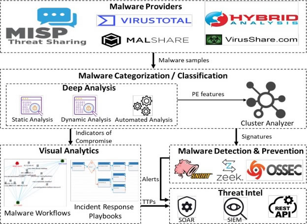
Figure 10. Architecture for the Analysis of Malware
Subsequently, a cluster analyzer examines the connections among clusters of malware. Malware clusters are a source of signatures that are utilized to supply intrusion detection and prevention systems, such as Snort and Zeek. Furthermore, Indicators of Compromise (IoCs) aid in comprehending malware TTPs graphically and enable a targeted response to each stage of an assault by employing Incident Response playbooks. Threat intelligence solutions, such as SOAR, security management, automation, and response APIs, utilize TTPs and alarms generated by malware detectors [43]. In order to effectively handle significant malware quantities, analyzing and detecting tools must meet the following criteria: precise identification of malicious software domains, automation to minimize analysis effort, efficient execution time, minimum usage of memory, consistent analysis to enable various security domains to sustain malware analysis, and resilience to noisy datasets such as network traffic or logs.
As of now, cyber analysts physically create lower-degree rules using detected IoCs for the purpose of design comparison (such as Sigma and Yara) plus correspondence. These techniques accurately detect established malware samples with a minimal number of false positives [44]. However, it is useless against polymorphic/metamorphic malware that has intricate pattern alterations, as well as zero-day malware. Malware analysts must exert a significant amount of work to create new rules for each new sample of malware. ML is always employed in addressing these constraints by facilitating the dynamic detection of abnormal virus behaviors. However, it frequently produces several inaccurate alerts when applied to real-world data. Machine learning is likewise plagued by problems of repeatability and robustness.
This study suggests employing TDA towards malware analysis and detection, with the aim of effectively aiding malware analysts in their everyday responsibilities. This decision is driven by the unique characteristics of TDA, including the ability to easily explore data by using topological graphs and persistence, stable performance against slight changes is ensured and the method is both reproducible and efficient in data classification for various fields such as infectious diseases, oncology, and renewable energy, as well as automation. Various topological data analysis (TDA) techniques have been employed, including persistence homology [45], TDA Mapper, and tomato, to effectively analyze and identify intricate malware in the presence or absence of disturbances. The objective was to achieve consistent results across multiple runs with minimal additional computational burden. In addition, it suggested using specific strategies to effectively deploy the most accurate models for large-scale malicious software detection. The literature also indicates that TDA Mapper, when integrated with PCA, is superior to PCA alone for clustering and uncovering concealed connections between malware clusters. Additionally, persistent diagrams outperform UMAP and t-SNE in efficiently identifying overlapping malware clusters. Furthermore, Random Forest and Decision Tree, when used in conjunction with t-SNE and PD, demonstrate greater effectiveness and resilience in handling datasets containing significant noise. Lastly, for improved performance and robustness, XGBoost and LightGBM are exclusively compatible with t-SNE. Therefore, malware researchers may utilize them effectively to enhance their routine operations of analyzing and detecting malware.
3. METHODOLOGY
We herein outline the TDA methods for the stability of functions in persistent homology.
Definition 3.1. [46] Topological Data Analysis (TDA) refers to a mathematical discipline that uses topological algebra and data science to discover the properties of data shape. Tools such as persistent homology are applied to discover multi–scale topological properties (e.g., connected components, holes) for uses in clustering, classification, and anomaly detection.
Definition 3.2. [47] Persistent Homology (PH) means a method scientists use in TDA to look for properties in a space that remain even as the filtration changes. It calculates a persistence diagram or barcode that captures the information about feature lifespans and aids in understanding the data at multiple scales.
Definition 3.3. [48] A simplicial complex consists of various simplices, including points, line segments, triangles, and shapes of high dimensions, stitched together, so that each simplex’s face is part of the complex and any interaction between two simplices is either void or shares a face. It allows shape and structure to be studied using a special combination of elements in algebraic topology, computational geometry, and data analysis.
Definition 3.4. [49] In the context of TDA, Big Data means data that is both complicated and high-dimensional and still contains worthwhile topological and geometric meaning. These kinds of datasets are studied using persistent homology, which detects key features such as voids, loops, and components found at multiple levels by repeatedly constructing simplicial complexes. TDA yields reliable and fixed summaries of data structure, able to display changes in volume using interpretable structures.
Definition 3.5. [50] Artificial Intelligence (AI) refers to systems that do complex mental tasks such as analyzing patterns and making decisions. AI supports Topological Data Analysis by drawing on topological summaries from persistent homology to add reliable shape-based details to the learning of data that is not easily structured.
Definition 3.6. [51] ML is an area within Artificial Intelligence that helps systems pick up on information from data to make predictions or decisions. In Topological Data Analysis, ML uses topological ideas, including persistent homology, to help it extract shape-based details from difficult and high-dimensional datasets.
4. RESULTS AND DISCUSSION
4.1. Homological functions
We now provide results from the study we conducted. If f, g, and two tame mappings from X to R are known, we are able to create two different potential functions by using sublevel set filtering on their images. The bottleneck distance is estimated by searching for the minimum of the maximum L∞-interval among corresponding points in both PDs. Here, all possible ways of bijectively matching points in the point sets of the PDs are examined. Those sets of diagonals Dgmkf and Dgmkg are shown by using (Dgmkf) ∪ ∆ and (Dgmkg) ∪ ∆ as point sets, as their coordinates are the same. The L∞-distance · ∞ starts by finding the absolute values for each member in a set of points and choosing the largest one, as seen in Equation 2 below:

Other helpful measures, such as p-Wasserstein [52] and Gromov-Hausdorff, are available for use as well. The variation among the functions f, ∞ which indicates the highest absolute difference between f(x) and g(x) over the set X, should be examined. They found that the distance between the top two most common classes was bounded, meaning that PD is stable.
Making persistence practical for machine learning requires kernels, Persistent Landscapes (PL), persistent entropy and persistent pictures. Although reaching cubic time complexity at peak, our method for PDs can be assimilated into a broad memory network. Tomato is software that was created to perform topological mode analysis [53]. For a given graph using X as a dataset, where the nodes are the points and edges join couples of points, this method designates a nonnegative parameter ˜f(xi) to every node xi. To find the important peaks of ˜f, the Persistence Diagram (PD) is used, giving us a way to find the peaks in f.
Seeing real data in practice shows there is always random noise and outliers, which may cause distance-based functions to fail entirely by making the results too unreliable. In fact, including even one outlying point in the point cloud can seriously disrupt the method by changing the distance function. Since the drawback cannot be corrected by regular estimation, we adopt a measure-theoretic approach and introduce DTM [54] as a solution. It remains constant against noise, and the finer sub-levels highlight many unique topological features. Significant effort has gone into understanding the main properties and estimation methods of the DTM. Still, the actual use of the distance-to-measure function produces disparities in choosing the variable m, which has partially been investigated but deserves more careful mathematical study.
4.2. Persistence Diagrams
PDs quickly show you the structure of a dataset. No matter how datasets originate from Rn, the true values cannot be determined, except if they result from a filtered set of states. An abstract SC is a tool from mathematics that looks like a graph. Each point on the 0-PD shown in the diagram indicates a connected home. Every 1-PD is made up of one single void. A two-punctured disk has each point standing in for a void, just like the interior of a football. The same pattern occurs for more detailed persistence diagrams. Each time a new simplex is included in the filtration, extra topological features occur. At time j, another simplex may be inserted to fill the hole, as topological holes can be born in interval i, disappear at j, and take up the time difference between the two moments. The point set (i-j) is what the 1-PD represents. To make persistence diagrams work with ML, they are incorporated into a vector representation. Experimenters prefer to integrate the PD into the persistent image as their main method of analysis [55]. The process steps 1 and 2 convert the birth and death in the plotings from plotting values into birth-persistence axes; step 3 applies a Gaussian to every point set and uses integration in a range to give a vector of weekly expected values. After that, the vector may be applied to several ML methods.
4.3. Persistence homology
Sometimes topology is called rubber sheet geometry, primarily because you could cut or bend any piece of rubber to appear like another similar type, keeping it intact. Figure 11 shows that a sphere and a cube are considered topologically the same. However, the sphere’s surface is distinctively dissimilar from a three-dimensional ball whose surface coincides with a sphere. Having homology in mind, we notice that the shape of the sphere borders free space in two dimensions, while the ball might be solid, so voids do not have the ball as their edge in three dimensions. We begin looking at homology by focusing on two quanta: we define β0 as the jammed material and β1 as the 1D holes. Our component’s contribution β0 is one once everything is connected.
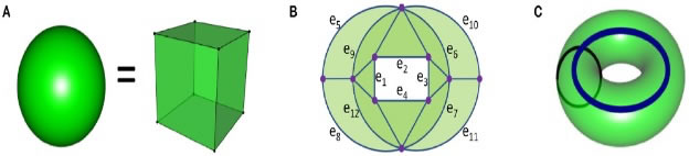
Figure 11. Equivalence in topologies
On the other hand, Homology will not therefore differentiate all items which are different topologically. For instance, the 1D circle and 2D surface in Figure 11 B, as well as the 3D solid torus, have a similar homology. (A) Both the filled-in ball and cube have a similar topology, hence similar homology. (B), (A) Having a topology border surface is the same as having a doughnut. In (C), a broad, bluish circle represents a 1D homological object that has created a firm doughnut with borders.
Approximating how connected and geometric datasets are has been achieved with the preceding DTM methods, using the intersection of balls centred on radius r [56]. For these approaches to work well, they depend on clear principles and a consistently formed shape over the data. That said, it is difficult to confirm these assumptions, so their usefulness is doubtful. Moreover, the main data structure usually depends greatly on the value chosen for r, as shown in Figure 12. At times, there is a possibility of having an incorrect topology of our dataset, as in Figure 12.
To overcome these difficulties in understanding multi-scale topological features in complex data sets, it is essential to invent new mathematical theories, so PH is an important tool within TDA. It introduces important frameworks and is based on effective algorithms to explore the ways in which family homology can reveal the inner workings of filtrations, the concept involving nested topological spaces or simplicial complexes found inside real number sets. Our discussion of TDA is centred around two kinds of filtrations. So, for metrics-based point cloud datasets, the vertex set of the filtered abstract simplicial complexes can be the same as the data point set. The Cech complex is one way to filter data, and it forms a connected chain of expanding balls around each data point. This way of persistent homology reflects the overall way the topological data is shaped as we vary the radii of the balls [57].

Figure 12. Predicted uncertainty of Big Data
4.4. Stable Functions in Persistence Diagrams
Many of the concepts involved seem to have universal relevance for algebraic stability in persistence theory. It is considered to have the power to play a significant role in improving stability several times. That is, it played a key role in ensuring the PDs are stable due to a filter put on the data sets after adding errors over the Gromov-Hausdorff metric. Topology and homology have a fundamental instability that is extremely important. If we add point sets to a topological space, both the number of elements and the Betti number are changed. It appears that these approaches are not suitable for studying data. One major point is that we should examine filtration made up of various spaces, rather than single rooms.

As a simple example in Expression 3, we could use the edge weights in a weighted graph to filter it. Any time we talk about scale, we can expect to see this phenomenon. PH reviews how the qualitative characteristics change when different parameters are selected. We see a regular decrease in the number of packages as we connect places that are increasingly far from one another. Single linkage clustering works exactly as this image shows. Different gaps may appear and disappear at different sizes depending on the dimension we are in.
The main point is that altering the different feature values from one parameter set can be seen simply by using a barcode or PD, as seen in Figure 13. Attempts have been made to apply these techniques to problem spaces with more dimensions, but that has been very challenging. More details about PH with many inside adaptations can be found in [41]. Next time, we’re going to look into persistence diagrams instead of barcodes. Every bar in this map matches a location, and as we move forward on the map, the x-axis indicates where we start with that bar, and the y-axis indicates its endpoint. With the left-side datapoints on the left, we create a barcode in the middle using the process. It reveals that the duration traits remain in the population. Each red bar indicates the amount of time during which component mergers took place; one-dimensional gaps are represented by blue bars. To make the persistence diagram (right), we set a single point for each bar, using its start and end as the corresponding x and y coordinates. You can notice the outlier, indicated by the blue dot off to the upper right in the dataset.
For this purpose, let’s suppose the function f is a map from a set called K to the set of real numbers R. The structure of our filtration leads us to refer to it as f1(−∞, α]. In particular, all simplices with values less than the others are included. Adding larger values to the dataset adds more simplices with lower function values, but they are added on their own. So, a collection of spaces is arranged one within the other, forming a filtration. We will define Xα as being the same as f1(−∞, α].

In this context of Expression 4, we study a metric space where all edges are less than α units apart. For every perturbed metric space, you get a special function g. As a result, a stable system has an output that only changes a little when the input is changed slightly. Even so, there are some limitations to this important outcome. Specifically, the bound uses the 1-norm, and when outliers appear, it can become very large. Lately, Wasserstein stability has gained attention since it provides more precise results, but its use is more limited than other results. Studies of stability now form a separate area, and we have learned about the different forms that stability can take.
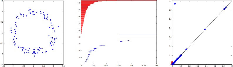
Figure 13. Perseverance succinctly
4.5. Persistence Homology to Machine Learning
ML designs have demonstrated remarkable accomplishments in computer vision, speech recognition, picture analysis, text analysis, and other related fields. Nevertheless, the utilization of these systems in complex high-dimensional environments has been greatly impeded due to the lack of appropriate feature representations. Conversely, features derived from conventional topological models retain the overall fundamental structural information, but they often diminish a significant amount of structural details and are infrequently employed for quantitative characterization. Recently, researchers have introduced PH as a novel method for representing topological properties at several scales. One can assess the inherent characteristics of topology. It has been observed that certain topological invariants persist for a longer duration in these SCs, whereas others diminish rapidly as the filtration parameters vary. These durations or durations of persistence of these constants are precisely correlated with features of geometry. In simple terms, long-lived Betti numbers typically indicate significant characteristics of considerable scale. By persisting throughout the filtration process, topological invariants can be quantified. Put simply, the lifespans or durations of these entities provide a relative geometric measure of the corresponding characteristics of topology. PH offers a highly promising method for representing structures and has been successfully implemented in several disciplines. These include shape recognition, network structure analysis, image analysis, data analysis [2], and computer vision.
Several software programs have been developed, such as JavaPlex, Perseus, Dionysus, jHoles, GUDHI, DIPHA, and the R-TDA package. Various techniques can be used to illustrate the results obtained by persistent homology (PH), such as PD (Persistent Diagram), PB (Persistent Barcode), PL (Persistent Landscape) [23], and persistent picture. Topological fingerprints can be derived from the persistent homology (PH) analysis of symmetric structures or structures with distinctive topological qualities. These fingerprints can then be utilized to quantitatively characterize the structures and functions of these objects [44]. However, as the systems become more intricate, it becomes increasingly difficult to construct models directly on the Persistent Barcode or Persistent Diagram. Another idea is to use machine learning to detect important patterns from topological data. Many industries, for example, image analysis, use Persistent-Homology-based Machine Learning (PHML) algorithms, along with time-series data analysis, computational biology, noise data and language analysis. However, PHML models face various challenges that are not present in geometric and classical topological models. These challenges include the development and creation of meaningful metrics, feature vectors, and kernels.
The distinctive structure of the PH result presents a significant obstacle to developing meaningful measurements. In order to address this issue, various distance measurements or metrics have been taken into account, such as Gromov-Hausdorff distance, Wasserstein Distance (WD), bottleneck distance, probability-measure-based distance, and Fisher information metric. The metric definitions are typically derived from PD, which can be regarded as a distribution of points in two dimensions. However, in contrast to typical point cloud data, PD points possess distinct topological importance. Short persistent times suggest topological characteristics that are negligible or noisy. While it may not hold true for a range of physical, chemical, and biological facts, there are instances where short-lived invariants carry significant physical significance. In contrast, long-lived topological generators are linked to intrinsic topological characteristics.
Moreover, the WD could be implemented to quantify the optimal correspondence between two probability distributions, while the bottleneck distance is a specific variant of the Wasserstein distance. The Wasserstein metric, Persistent Diagrams (PDs), exhibit completeness and separability. Fréchet variance and mean, which extend this concept to a broader metric space, could also be applied to probability distributions to facilitate probabilistic analysis. The Wasserstein distance does not directly punish the difference in cardinality between two probability distributions. A distance function based on probability measures to consider changes in tiny persistence and cardinality. Additionally, it allows for the incorporation of statistical structure through Frchet means and variances and offers a system for classification. Each of these metrics and distance measurements can be applied to the building of kernels and subsequently to ML frameworks.
PDs/PBs could be used to generate topological features. A straightforward approach to generating features based on PD/PB includes gathering their analytical characteristics, including total, average, variance, maxima, minima, etc. Features can include special aspects of topology, like the total Betti number at a specific filtration value. Additionally, [15] suggests plots that represent characteristics of the relevant ring of functions and serve as topological features for the categorization of digit numbers. Tropical coordinates, which are stable in relation to WD, are significant topology characteristics in the space of barcodes. Nevertheless, all of these solutions solely utilize incomplete data from PB. The binning methodology, proposed and further developed by, provides a more systematic method for building features of topology vectors from PDs and PBs. The fundamental concept involves dividing the PB/PB into distinct attributes that could be subsequently combined into a feature vector.
In addition, an alternative approach to creating features from PDs/PBs involves constructing functions of persistence, discretizing them into components, and then concatenating them into a vector. These enduring functions encompass the Betti number that persists, the Betti function that persists, the PLs, the persistent surface, and so on. In addition, a visual representation of PDs/PBs has proven to be highly valuable in the field of drug design. This model decomposes biomolecular structure into element-specific models, from which every model is denoted by a feature vector obtained by a binning technique. Instead of immediately utilizing these feature vectors, a method is suggested to methodically combine them into an image representation by stacking them together. The approach effectively showcases the immense potential of persistent representation. Finally, [46] has developed a permanent path and signature feature framework. The barcode findings are integrated within a durable pathway in this architecture. This tenacious path is subsequently converted into a tensor series, which is then represented as a feature vector. Importantly, it is noted that new methods of topological representations have shown great potential for PHML models. These methods can incorporate additional structural information, such as persistent local homology, element-specific PH, and multidimensional PH. Statistically speaking, if an expansive feature vector is employed to depict the topology characteristics of PBs/PDs, the PHML frameworks could likewise be affected by the curse of dimensionality. When facing this scenario, it is important to take into account methods for selecting variables and applying regularisation.
The fundamental concept behind PHML is to derive topological characteristics within datasets while utilizing persistent homology, then subsequently integrate the characteristics within ML techniques, encompassing either supervised or non-supervised learning methodologies. Figure 14 demonstrates that PHML could be segmented to produce four distinct stages: SC creation, analysis of PH, extraction of features of topology, and topological ML. Various data types are associated with distinct simplicial complexes. By selecting an appropriate filter setting, PH analysis can be carried out using specialized software. The output of Persistent Homology is converted into Feature Vectors (FV), distance measurements, or specialized kernels. These are then integrated with supervised or non-supervised ML techniques.
Classification is a discipline in Machine Learning (ML) where data with unknown categories is labeled using existing data labels. Classification encounters difficulties such as dealing with a large number of features, the presence of irrelevant information, and uneven data distribution. TDA has effectively reduced dimensionality and shown resilience to noise by deducing the primary topological data set. Nevertheless, the methodology of utilizing TDA to identify unbalanced datasets remains unexplored. This study presents a technique that relies only on TDA to categorize datasets that are both unbalanced and noisy. The core concept is to offer multifaceted and multiple-sized neighborhoods surrounding any unmarked point. Topology constants calculated via persistent homology are utilized to identify suitable neighborhoods. We utilize the concept of neighborhoods to transmit labels from places that have been labeled to points that have not been labeled.
Using Persistent Homology (PH), TDA can identify core geometric features in collections of data structures that are formed one at a time by increasing the threshold value. The values at which each phase is created and ends are what show its topological properties. The difference in numbers between those born and those who perish is called the persistence of a topological characteristic. Barcodes and persistence diagrams are used to show the development of the simplicial structure. With respect to the connection between PH and the classification issue, the current strategy involves the use of hybrid TDA+ML approaches. These methods integrate topological characteristics with a standard ML classifier. Topological identifiers are often constructed using vectorized or summarised persistence diagrams and barcodes. Some examples of hybrid approaches that combine TDA with ML are TDA plus SVM for classifying images, TDA plus k-NN, TDA plus CNN, as well as TDA plus SVM for time-series categories [48]. The combination of Self-Organized Maps and PH tools was used to cluster and categorize time series data in the financial area.
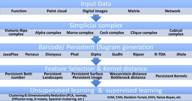
Figure 14. PHML Flowchart Model
The barcode component of PH is a tool used as a topology signature to reveal structure out of datasets. As far as homology discovers the topology in data and not its geometry, persistent homology, on the other hand, operates by detecting geometrical shapes. Machine learning as a technique could be implemented in groups of PDs to detect datasets with discrete features. The majority of ML algorithms utilize input vectors. Several methods exist to construct vector spaces from persistent homology. Figure 15 illustrates one such method used to generate a vector through persistence images.

Figure 15. Vectorization of a persistent diagram by use of persistence images
To begin, a persistent diagram initially gets pivoted by 45◦ after which the diagonal emerges as the horizontal axis. Hence, the plane axis denotes the birth interval, while the vertical axis denotes the persistence, which equals death minus birth. As a result, heat maps get generated through a Gaussian-distribution of every point (see third panel). The Gaussian distribution height is designated using colors within the heat map, and it's reliant on the persistent feature. Points near the diagonal are regarded as noise and hence not given color concentration. Therefore, the heat map bottom shall be consistently marked with the color denoting the lowest intensity, which is blue.
By way of explanation, those points adjacent to the diagonal will have very minimal to no impact on the heat map. Also, note that those points away from the diagonal within the first panel represent those properties endowed with the largest persistence from the 2nd panel. Hence, as for the heat map within the third panel is assigned a strong color, yellow in this case. As we can see on the 4th panel, the heat map is detached through a subdivision of heat maps into n x n squared shapes, from which every square color is proportionate to the means of respective squared shapes within these heat maps. As for these detached heat-maps on the fourth section, the yellow section within the third section relative to extremely persistent properties gets portioned into the two square-shaped components, as yellowish squares located atop the row within the heat-map with a greater portion over the pink ones adjacent on the same row. Within the last section, the n2-D vector is generated through the integration of detached heat-maps rows.
The primary goal of persistent homology is to analyse the emergence and diminishing of attributes of topology on a topological space while the scale value, often a radius, gradually changes. This process is referred to as filtration. In several simplicial complexes, the simplices are defined based on their closeness as measured by a distance function. A filtration F on an SC K is created by selecting a set εK of non-negative values 0 < ϵ0 < ϵ1 <…< ϵn, where each complex Ki corresponds to a specific value ϵi. A filtration may be defined as a process of constructing the entire simplicial complex K by sequentially organizing a ”family” of sub-complexes based on certain criteria.
The filtration measure assigned to q-simplex: Consider K as a filtered SC, where εK represents its collection of filtration values. Consider σ, which is a q-simplex in the set K. If σ belongs to Kj but does not belong to Kj−1, then ξK(σ) is defined as εj, the filtration value of σ. It should be noted that τ is less than or equal to σ, which implies that ξK(τ ) is less than or equal to ξK(σ), as shown in Figure 16.

Figure 16. The filtration values associated with the simplicies
Consider Rn as a real space and P as a finite subspace contained within Rn. Let P be partitioned into two sub-spaces such that P equals S union X, where S represents the training dataset and X represents the testing dataset. Given L is a set of labels, defined as L = l1, ..., lN. Let T be the connection space, denoted as T = (p, l) : p ∈ P, l ∈ L. T is composed of two disjoint linkage sets, TS and TX, T = TS ∪ TX, TS and TX correlating to both S and X. The marking Y, denoted as li|(xi, li) ∈ TX, represents the markings listed to every attribute of X in the similarity set TX. The classifying issue may be characterized as the task of predicting an appropriate label, l ∈ L denoted as l, from a set of possible labels, denoted as L, for each input, denoted as x, from a collection of inputs, denoted as X, x ∈ X. This prediction is made under the assumption that the association set, denoted as TX, is not known.
This section introduces a classification approach that is based on Topological Data Analysis (TDA). In general, a refined SC K is constructed across P to provide connections between datapoints. The suggested technique relies on the premise that there is a subset of a complex Ki ⊂ K present in the filter, where the simplices of Ki accurately describe the topology of the data. The inclusion of a point set v0, v1, ..., vq ⊂ P in a q-simplex σ ∈ K indicates a connection of like or dislike amongst the points v0, v1, ..., vq. The suggested technique utilizes this implicit link among data to transfer markings from marked points to unmarked points.
The mapper algorithm concept was initially proposed by [51], and it is predicated upon the notion of partly grouping the dataset based on a series of functions built around this dataset. At a macroscopic level, the mapper graph represents the overall organization of this dataset. Consider S as a subset of Rk, representing a point-cloud space containing high dimensional features. A cover of set S in Rk is an assemblage of open sets U = Ui where S is a subset of the union of all Ui. In the traditional mapper architecture, the process of getting the covering of set S is directed by a collection of scalar functions specified on S, which are often known as filter functions. To make it simpler, we’ll assume the mapper is built using just a filter function f which turns every element from S into an element from R. If we produce a U of S, we can group components in Vl of f(S) together using clustering to generate clusters for U. We will use these clusters to decorate and support the objects in place for set S. The N1(U) nerve is shown as a graph, with the number one representing the dimensionality. Every node i within the set N1(U) signifies the covering component Ui, while there is an existence of an edge in the middle of nodes i and j given that the intersection of Ui and Uj is non-empty. If U is created in the manner described, by clustering the inverse images of a filtration function f, then it is a 1-dimensional nerve, represented as M = M(S, f):= N1(U), which represents (S, f), our mapper graph.
Figure 17 depicts a point cloud that serves as an illustrative example, consisting of two circles stacked within each other. The height function f mapping the set S to R is included.
Given the cover V = V1,…, V5 of f(S) consisting of five intervals (Figure 17), for any value of l (where one is less than or equal to l and l is less than or equal to 5), the inverse function f−1(Vl) creates a collection of clusters that are subsets of S. The clusters constitute the components of the covering U of S. Figure 17 (left) demonstrates that the cover components of U are enclosed by the twelve rectangles on the plane. For example, when the cover f−1(V1) is applied, it results in a cole cover component U1 of S. This cover element U1 then generates node 1 in the mapper graph of S. The function f−1(V2) results in the creation of three cover components, namely U2, U3, and U4, which are then transformed into nodes 2, 3, and 4. Given that the intersection of U1 and U2 is not empty, there is a connection linking node one and node two.

Figure 17. A topological representation of a point cloud displaying two concentric rings
The mapper graph in Figure 17 (right) encompasses the two circular constructions seen on the left. In the PD, orange spots are for 1-dimensional persistent features, and blue points indicate 0-dimensional persistent features. Those points sitting on the horizontal dotted line are characterized by their persistence during the whole filtering and the absence of a death threshold.
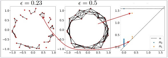
Figure 18. VR complexes and persistence diagram of the point cloud
TDA Mapper is a method that summarizes data points in a given data set X by analyzing the net of the cluster of linked elements within the open sets {f−1(Ui)i∈I}, such that the function f mapping the set X to Rn results to a function that acts as a continuous filter or lens. It maps each element Ui in the indexing set I to an element U: Ui ∈ U. The preimages of Ui under the function f−1 are also considered. A neuron is a mathematical structure composed of nodes as well as edges, which capture significant geometrical characteristics within the initial dataset, such as voids, elements, and branching. This TDA Mapper graph is represented by the notation M(X, U, f), hence calculated in the following manner:
Apply the filter/lens function f to the dataset X in order to map it into the Euclidean space Rn: f: X → Rn.
Enclose the depiction of f(X) of our data set X contained in a space Rn within a cluster of open sets U = {Ui}i∈I. The value of U is equal to the function f multiplied by the constant.
Apply a clustering method, such as k-nearest neighbor or density-based, on each preimage f−1(Ui) to obtain ip clusters Ci1, ..., Cip. Compute the cryptographic hash function output for the i-th input.
Construct the nerve by considering a series of all collections {Ci1, ..., Cip} given all the vertices vjk ∈ Cik}. Vertex vjk is connected to vertex vkl by an edge if and only if the set difference between Cjk ∩ Ckl ̸= ∅.
This graph of the TDA Mapper requires a meticulous selection of its different parameters. For instance, the functionality of the filter/lens relies on the characteristics of the datasets, and the grouping technique has to be supplied in order to calculate pre-images. The algorithm of the TDA Mapper could be computed in polynomial time and can be parallelized without compromising the accuracy of the findings [53].
4.6. Persistent Homology in Cybersecurity Systems
Compared to Mapper, which generates a graph visualization of elements of interest in a data set, persistent homology technology reveals a vivid numerical data shape, which cannot be revealed by conventional statistical techniques like variance and mean. Persistent homology vectors the data sets to form the Betti sequence. Log analysis is among the tasks of an enterprise cybersecurity professional. However, this is an uphill task since it involves millions of logs collected in seconds. Among these logs could be malicious keying of inappropriate credentials, true negatives, and malware. Investigation of these logs becomes a priority to be up to date with current threats, emerging threats, as well as coming up with better firewall rules. TDA is therefore fundamental in alert investigation, generating interestingly new, insightful knowledge about the threat landscape.
Nearly all digital government infrastructure comprises complex network devices encompassing different protocols. Besides, security and reliability of such systems need to be assured, and this requires a rapid response to every cyber event, whether false-positive or false negative [34]. Enterprise cyber-systems implement access control for all endpoint devices in the network, including Internet-of-Things (IoT) devices.
Stateful firewalls and IDPS are, in most cases, used in defending networked enterprises through evaluation, identification, and filtering bad reputation packets. The rules could include references to non-benign IPs to be blocked or TCP/UDP protocol events over a time period. Every time these rules get triggered by unusual alerts, security devices log these alerts detailing the violated preset rules [21]. These events usually capture no encapsulated packets, which triggered the incidents, despite having information of interest. Thus, investigations are always based on metadata, while analyzing the packets transmitted is an impossibility. Because of the extremely high volumes of Network traffic when captured, which is Big Data in nature, it can therefore be analyzed in PCAP files or data streams. PCAP files capture and process network packets while data traffic gets processed instantaneously.
The author [56] constructed simplicial complicated filtrations using Windows Sysmon records. He constructed a filtration of SC in the following manner: given a set of logs that he categorized as benign or anomalous. The 0-simplices are distinct identifiers seen in the logs, including file names, IP addresses, ports, and process IDs. When the filter first showed up in the logs, that’s when it was entered. Every time 2 zero-simplices interrelate in a log-entry, he appended 1-simplices. For instance, when two IP addresses are connected via a network, or when one process starts another. At the moment of the relevant log entry, the 1-simplex enters the filtration. After experimenting, he discovered that the addition of induced 2-simplices had no discernible effect on performance. After that, he computed the logs’ persistence diagram and persistence images. An illustration of this can be found in Figure 19.
He tried with various persistence image resolutions and discovered that there was little to no effect. He also took into account the hypergraph Laplacian and the graph Laplacian’s spectrum as features. He obtained a graph by taking into account the zero and one-simplices of the ending SC within the filter. He calculated its Laplacian spectrum, which served as a feature vector. In a similar manner, he could create a hypergraph from log entries and use its spectrum as a feature vector to produce a hypergraph Laplacian. It is important to record that a hypergraph is a more general form of an SC because it does not require every sub-border to be in the hypergraph. He could construct a hypergraph by appending log entries to hyperedges. As an illustration, a process ID that initiated network-based events linking a single IP address with a port to a separate IP address and port may constitute one hyper-edge, resulting in a hyperedge with five nodes. As a baseline, he lastly put the count vectorization approach into practice[57]. Our algorithms are well-suited for this vector since it is frequently employed for automated anomaly identification in log events. The term ”counts” refers to this baseline. For every feature vector, he employed a ten-fold multivariate random forest as their classification parameters.

Figure 19. Windows logs incorporated into an SC
Two distinct private datasets were used for conducting the experiments. The dataset comprises around 1600 instances of a Windows system, with each instance representing about 3-minute events, which have been recorded while utilizing the open-source Logging Made Easy (LME) project. Every run is characterized by either normal or abnormal system activities. The dataset involved the performance of either clean software (baseline) or malicious software (anomalous) activities. Every software run on the dataset was distinct for each execution. There are a total of 320 runs, divided into 160 baseline runs and 160 ’attack’ runs. The attack runs include fileless attacks, which utilize valid system tools to carry out malicious activities, attacks that use already installed files on the hosts, assuming the malicious software has infiltrated the system through phishing attacks or related means, and attacks that involve downloading malware from a remote source prior to their installation. Every run in the dataset is included without any obfuscation, but also with four different obfuscation techniques applied to key descriptors in the logs, such as Base64 and Caesar cipher encodings. The dataset contains a greater range of types of attacks in the malicious datasets. However, it contains fewer distinct attacks. The study involved comparing four distinct techniques: the count’s baseline, persistent homology (specifically the 0 and 1-persistence pictures), the graph Laplacian spectrum, and the spectrum of the Hypergraph Laplacian (HL). Furthermore, all tests were conducted utilizing two distinct logsets, denoted as constructs. Construction 1 utilized process-created and network-based activity logs, whereas the second Construction incorporated process creation, process termination, file creation, and network-based event logs. The mean accuracy, precision, recall, and F1 scores (with error boundaries) were computed for each trial using a ten-fold cross-examined random forest. Figure 20 illustrates the relationship between the count of logs and the validity of our frameworks. It is expected that when we increase the number of logs, our models could perform better. Specifically, in our dataset, Construction 2 consistently achieves a 4%-5% higher accuracy compared to Construction 1. The disparity is less pronounced in our dataset, although it remains noteworthy in some measurements and methodologies. The back-and-forth is that the increase in the count of logs results in higher computational complexity. If the aim is to execute the proposed techniques as instantaneously as feasible, an option is to use minimal types of logs. This decision may sacrifice some performance but will lead to faster computation times.

Figure 20. Baseline vector Counts(C), PH, GL, HL, and both Counts Vector and Graph Laplacian
Classification accuracy of anomalous logs is evaluated across all data sets, constructions, and feature encapsulations. The outcomes are shown for the PH with the 0th and first dimensions (PH), the counts baseline vector (C), the GL, and the Hypergraph Laplacian (HL), and for the combination of the counts’ vector and graph Laplacian (C+GL). The classification parameter is a random forest that has been cross-validated using a 10-fold technique.
Our dataset shows that counts perform better than persistent homology by around 6%, and are somewhat superior to the graph and HL. Counts in Data Set Two are equivalent to PH; however, they are surpassed by the graph and hypergraph Laplacians in terms of performance. The fundamental outcome of this study should be regarded as the ability of the examined topological and spectral approaches to operate at a level that is comparable to or even above a conventional baseline. Count vectors incorporate specific information regarding the characteristics of various event logs, whereas topological and spectral feature vectors just rely on the inherent overall structure of the logs. The fact that our methodologies can match the numbers’ baseline indicates that the information structure alone is barely identifying the abnormal behavior. That this will indeed be the case was not guaranteed. Given that our approaches are unaffected by the obfuscation techniques used, our dataset's higher overall findings are probably due to certain similarities that exist between the train and test sets due to how the data was obfuscated. We should remember that this principle works for all methods, so examining different techniques becomes very useful. Besides, the hypothesis was formulated that distinct views were obtained from the counting procedure and the topological/spectral analysis. To determine these scenarios, we designed a novel feature vector by merging the count vector with the graph Laplacian. This feature vector is created by blending the two; it had superior performance in nearly all metrics, either matching or surpassing almost every other method, confirming our theory.
5. CONCLUSION
It is generally not easy to describe the topological and geometric characteristics in point-set topological spaces. Research in TDA looks at the possibility of finding accurate measures of geometry and topology in big datasets when the data is kept in a global structure. This question introduces another problem: the estimates are useful only if we can determine if the constants are stable, despite no changes in data inputs, for instance, the Hausdorff distance function when the data exhibits noise, or even when a little noise is added to the point-cloud datapoints. This could happen if these properties are considered in topologically invariant compact subsets of X, which requires very stringent and restrictive assumptions to obtain well-defined shapes that can be drawn from the data in the compact subsets. In connection with this, the purpose of this study is to examine the stability of functions found in persistent homology. In addition, only a small amount of work exists in calculating Cybersecurity information with persistent homology, as previous studies only leveraged Mapper, another aspect of TDA. In this study, we have proposed an integrated artificial intelligence framework for the stability of functions by tracking the stability of algorithms. Cyber-threat detection and cyber-attack prediction are possible within the cybersecurity data sets, using Persistent Homology.
DATA AVAILABILITY STATEMENT
The data presented in this study are available on request from the corresponding author.
CONFLICTS OF INTEREST
The authors declare that they have no conflicts of interest in this work.
REFERENCES
[1] F. Verhulst, Henri Poincaré. Boston, MA: Springer US, 2012. doi: 10.1007/978-1-4614-2407-9.
[2] H. Poincaré, and J. Stillwell, “Papers on Topology: Analysis Situs and its Five Supplements,” Am Math Soc Math Soc, vol. 37, p. 228, 2010.
[3] L. E. J. Brouwer, “Beweis der Invarianz der Dimensionenzahl,” Math Ann, vol. 70, no. 2, pp. 161–165, Jun. 1911, doi: 10.1007/BF01461154.
[4] E. Betti, “Sopra gli spazi di un numero qualunque di dimensioni,” Ann di Mat Pura ed Appl, vol. 4, no. 1, pp. 140–158, Jul. 1870, doi: 10.1007/BF02420029.
[5] J. W. Alexander, “A Proof of the Invariance of Certain Constants of Analysis Situs,” Trans Am Math Soc, vol. 16, no. 2, p. 148, Apr. 1915, doi: 10.2307/1988715.
[6] P. Hilton, “A Brief, Subjective History of Homology and Homotopy Theory in This Century,” Math Mag, vol. 61, no. 5, pp. 282–291, Dec. 1988, doi: 10.1080/0025570X.1988.11977391.
[7] B. Srinivasan and J. D. Sally, Eds., Emmy Noether in Bryn Mawr. New York, NY: Springer New York, 1983. doi: 10.1007/978-1-4612-5547-5.
[8] G. Carlsson, “Topology and data,” Bull Am Math Soc, vol. 46, no. 2, pp. 255–308, Jan. 2009, doi: 10.1090/S0273-0979-09-01249-X.
[9] T. Davies, “Persistence-Based Summaries for Data Analysis with Applications to Cyber Security,” Univ Southampton, Dr Thesis, p. 164, 2023.
[10] P. Bubenik, M. Hull, D. Patel, and B. Whittle, “Persistent homology detects curvature,” Inverse Probl, vol. 36, no. 2, p. 025008, Feb. 2020, doi: 10.1088/1361-6420/ab4ac0.
[11] J. Franklin, “The elements of statistical learning: data mining, inference and prediction,” Math Intell, vol. 27, no. 2, pp. 83–85, Mar. 2005, doi: 10.1007/BF02985802.
[12] Y. LeCun, Y. Bengio, and G. Hinton, “Deep learning,” Nature, vol. 521, no. 7553, pp. 436–444, May 2015, doi: 10.1038/nature14539.
[13] P. Bubenik and P. Dłotko, “A persistence landscapes toolbox for topological statistics,” J Symb Comput, vol. 78, pp. 91–114, Jan. 2017, doi: 10.1016/j.jsc.2016.03.009.
[14] F. Chazal, D. Cohen‐Steiner, L. J. Guibas, F. Mémoli, and S. Y. Oudot, “Gromov‐Hausdorff Stable Signatures for Shapes using Persistence,” Comput Graph Forum, vol. 28, no. 5, pp. 1393–1403, Jul. 2009, doi: 10.1111/j.1467-8659.2009.01516.x.
[15] M. K. Chung et al., “A Unified Statistical Approach to Deformation-Based Morphometry,” Neuroimage, vol. 14, no. 3, pp. 595–606, Sep. 2001, doi: 10.1006/nimg.2001.0862.
[16] F. Chazal, L. J. Guibas, S. Y. Oudot, and P. Skraba, “Persistence-Based Clustering in Riemannian Manifolds,” J ACM, vol. 60, no. 6, pp. 1–38, Nov. 2013, doi: 10.1145/2535927.
[17] T. Florian, H. Carl, K. Hedvig, and K. Danica, “Topological constraints and kernel-based density estimation,” Adv Neural Inf Process Syst, vol. 25, 2012.
[18] C. S. Pun, S. X. Lee, and K. Xia, “Persistent-homology-based machine learning: a survey and a comparative study,” Artif Intell Rev, vol. 55, no. 7, pp. 5169–5213, Oct. 2022, doi: 10.1007/s10462-022-10146-z.
[19] Edelsbrunner, Letscher, and Zomorodian, “Topological Persistence and Simplification,” Discrete Comput Geom, vol. 28, no. 4, pp. 511–533, Nov. 2002, doi: 10.1007/s00454-002-2885-2.
[20] E. Munch, M. Shapiro, and J. Harer, “Failure filtrations for fenced sensor networks,” Int J Rob Res, vol. 31, no. 9, pp. 1044–1056, Aug. 2012, doi: 10.1177/0278364912451671.
[21] V. Snášel, J. Nowaková, F. Xhafa, and L. Barolli, “Geometrical and topological approaches to Big Data,” Futur Gener Comput Syst, vol. 67, pp. 286–296, Feb. 2017, doi: 10.1016/j.future.2016.06.005.
[22] V. Divol and T. Lacombe, “Understanding the topology and the geometry of the space of persistence diagrams via optimal partial transport,” J Appl Comput Topol, vol. 5, no. 1, pp. 1–53, Mar. 2021, doi: 10.1007/s41468-020-00061-z.
[23] P. J. Chocano, M. A. Morón, and F. R. Ruiz del Portal, “Computational approximations of compact metric spaces,” Phys D Nonlinear Phenom, vol. 433, p. 133168, May 2022, doi: 10.1016/j.physd.2022.133168.
[24] W. S. Admass, Y. Y. Munaye, and A. A. Diro, “Cyber security: State of the art, challenges and future directions,” Cyber Secur Appl, vol. 2, p. 100031, 2024, doi: 10.1016/j.csa.2023.100031.
[25] I. Jada and T. O. Mayayise, “The impact of artificial intelligence on organisational cyber security: An outcome of a systematic literature review,” Data Inf Manag, vol. 8, no. 2, p. 100063, Jun. 2024, doi: 10.1016/j.dim.2023.100063.
[26] A. Berentsen, “Aleksander Berentsen Recommends ‘Bitcoin: A Peer-to-Peer Electronic Cash System’ by Satoshi Nakamoto,” in 21st Century Economics, Cham: Springer International Publishing, 2019, pp. 7–8. doi: 10.1007/978-3-030-17740-9_3.
[27] J. Lewis, “Economic impact of cybercrime -No Slowing Down,” McAfee, St Cl, vol. 2, 2018.
[28] A. Martin, J. Hernandez-Castro, and D. Camacho, “An in-Depth Study of the Jisut Family of Android Ransomware,” IEEE Access, vol. 6, pp. 57205–57218, 2018, doi: 10.1109/ACCESS.2018.2873583.
[29] B. T. Fasy, F. Lecci, A. Rinaldo, L. Wasserman, S. Balakrishnan, and A. Singh, “Confidence sets for persistence diagrams,” Ann Stat, vol. 42, no. 6, Dec. 2014, doi: 10.1214/14-AOS1252.
[30] L. N. Tidjon, M. Frappier, and A. Mammar, “Intrusion Detection Systems: A Cross-Domain Overview,” IEEE Commun Surv Tutorials, vol. 21, no. 4, pp. 3639–3681, 2019, doi: 10.1109/COMST.2019.2922584.
[31] A. Zomorodian and G. Carlsson, “Computing Persistent Homology,” Discrete Comput Geom, vol. 33, no. 2, pp. 249–274, Feb. 2005, doi: 10.1007/s00454-004-1146-y.
[32] F. Chazal and B. Michel, “An Introduction to Topological Data Analysis: Fundamental and Practical Aspects for Data Scientists,” Front Artif Intell, vol. 4, Sep. 2021, doi: 10.3389/frai.2021.667963.
[33] M. E. Aktas, E. Akbas, and A. El Fatmaoui, “Persistence homology of networks: methods and applications,” Appl Netw Sci, vol. 4, no. 1, p. 61, Dec. 2019, doi: 10.1007/s41109-019-0179-3.
[34] G. F. Monkam, M. J. De Lucia, and N. D. Bastian, “Preprocessing Network Traffic using Topological Data Analysis for Data Poisoning Detection,” in 2023 IEEE Conference on Dependable and Secure Computing (DSC), IEEE, Nov. 2023, pp. 1–8. doi: 10.1109/DSC61021.2023.10354143.
[35] B. M. Balachandran and S. Prasad, “Challenges and Benefits of Deploying Big Data Analytics in the Cloud for Business Intelligence,” Procedia Comput Sci, vol. 112, pp. 1112–1122, 2017, doi: 10.1016/j.procs.2017.08.138.
[36] A. Omorede, J. F. Prados-Castillo, and A. C. Casas-Jurado, “Researching entrepreneurship using big data: implementation, benefits, and challenges,” Int Entrep Manag J, vol. 21, no. 1, p. 85, Dec. 2025, doi: 10.1007/s11365-025-01100-w.
[37] X. Meng, Y. Pei, and H. Takagi, “Evolutionary Multi - Modal Optimization Using Persistence-Based Clustering in Riemannian Manifolds,” in 2024 IEEE Congress on Evolutionary Computation (CEC), IEEE, Jun. 2024, pp. 1–8. doi: 10.1109/CEC60901.2024.10612013.
[38] F. Chazal, D. Cohen-Steiner, and Q. Mérigot, “Geometric Inference for Probability Measures,” Found Comput Math, vol. 11, no. 6, pp. 733–751, Dec. 2011, doi: 10.1007/s10208-011-9098-0.
[39] D. Barnes, L. Polanco, and J. A. Perea, “A Comparative Study of Machine Learning Methods for Persistence Diagrams,” Front Artif Intell, vol. 4, Jul. 2021, doi: 10.3389/frai.2021.681174.
[40] J.-D. Boissonnat, F. Chazal, and B. Michel, “Topological Data Analysis,” 2022, pp. 247–269. doi: 10.1007/978-3-030-96173-2_9.
[41] G. Rote and G. Vegter, “Computational Topology: An Introduction,” in Effective Computational Geometry for Curves and Surfaces, Springer Berlin Heidelberg, pp. 277–312. doi: 10.1007/978-3-540-33259-6_7.
[42] P. Niyogi, S. Smale, and S. Weinberger, “A Topological View of Unsupervised Learning from Noisy Data,” SIAM J Comput, vol. 40, no. 3, pp. 646–663, Jan. 2011, doi: 10.1137/090762932.
[43] V. Patrangenaru, P. Bubenik, R. L. Paige, and D. Osborne, “Challenges in Topological Object Data Analysis,” Sankhya A, vol. 81, no. 1, pp. 244–271, Feb. 2019, doi: 10.1007/s13171-018-0137-7.
[44] K. Xia, Z. Li, and L. Mu, “Multiscale Persistent Functions for Biomolecular Structure Characterization,” Bull Math Biol, vol. 80, no. 1, pp. 1–31, Jan. 2018, doi: 10.1007/s11538-017-0362-6.
[45] A. Adcock, E. Carlsson, and G. Carlsson, “The Ring of Algebraic Functions on Persistence Bar Codes,” Apr. 2013. http://arxiv.org/abs/1304.0530
[46] I. Chevyrev, V. Nanda, and H. Oberhauser, “Persistence Paths and Signature Features in Topological Data Analysis,” IEEE Trans Pattern Anal Mach Intell, vol. 42, no. 1, pp. 192–202, Jan. 2020, doi: 10.1109/TPAMI.2018.2885516.
[47] B. Okelo and A. Onyango, “Persistent Homology and Artificial Intelligence Analysis of COVID-19 in Topological Spaces,” DS J Digit Sci Technol, vol. 2, no. 3, pp. 1–8, Sep. 2023, doi: 10.59232/DST-V2I3P101.
[48] L. M. Seversky, S. Davis, and M. Berger, “On Time-Series Topological Data Analysis: New Data and Opportunities,” in 2016 IEEE Conference on Computer Vision and Pattern Recognition Workshops (CVPRW), IEEE, Jun. 2016, pp. 1014–1022. doi: 10.1109/CVPRW.2016.131.
[49] D. Cohen-Steiner, H. Edelsbrunner, and J. Harer, “Stability of Persistence Diagrams,” Discrete Comput Geom, vol. 37, no. 1, pp. 103–120, Jan. 2007, doi: 10.1007/s00454-006-1276-5.
[50] R. Kindelan, J. Frías, M. Cerda, and N. Hitschfeld, “A topological data analysis based classifier,” Adv Data Anal Classif, vol. 18, no. 2, pp. 493–538, Jun. 2024, doi: 10.1007/s11634-023-00548-4.
[51] R. P. Singh, N. O. Malott, B. Sauerwein, N. Mcgrogan, and P. A. Wilsey, “Generating High Dimensional Test Data for Topological Data Analysis,” 2024, pp. 18–37. doi: 10.1007/978-981-97-0316-6_2.
[52] E. Purvine et al., “Experimental Observations of the Topology of Convolutional Neural Network Activations,” Proc AAAI Conf Artif Intell, vol. 37, no. 8, pp. 9470–9479, Jun. 2023, doi: 10.1609/aaai.v37i8.26134.
[53] M. Hajij, B. Assiri, and P. Rosen, “Parallel Mapper,” May 2020. http://arxiv.org/abs/1712.03660
[54] A. F. Zobaa and T. J. Bihl, Eds., Big Data Analytics in Future Power Systems. Boca Raton : Taylor & Francis, a CRC title, part of the Taylor &: CRC Press, 2018. doi: 10.1201/9781315105499.
[55] L. Zhang and G. B. White, “Analysis of Payload Based Application level Network Anomaly Detection,” in 2007 40th Annual Hawaii International Conference on System Sciences (HICSS’07), IEEE, Jan. 2007, pp. 99–99. doi: 10.1109/HICSS.2007.75.
[56] B. Kuskonmaz, R. Wisniewski, and C. Kallesøe, “Topological Data Analysis-Based Replay Attack Detection for Water Networks,” IFAC-PapersOnLine, vol. 58, no. 4, pp. 91–96, 2024, doi: 10.1016/j.ifacol.2024.07.199.
[57] R. Winding, T. Wright, and M. Chapple, “System Anomaly Detection: Mining Firewall Logs,” in 2006 Securecomm and Workshops, IEEE, Aug. 2006, pp. 1–5. doi: 10.1109/SECCOMW.2006.359572.
BIOGRAPHIES OF AUTHORS

Onyango Allan Onyango Received his master’s degree in Pure Mathematics in 2023. He has 4 years of professional experience in Computer Networks. He is presently pursuing his PhD in Pure Mathematics from JOOUST and Erasmus Mundus joint master’s degree in Applied Cybersecurity at Kadir Has University, Turkey and Berlin University of Applied Sciences, SRH (Germany). His research interests include: Machine Learning, TDA, Network Security, Computer Networks, Operating Systems, and Cybersecurity Management. He has published in International Journals, including: DS-DST, JDSIS, and TFSS. He can be contacted at email: onyango.onyangoa@gmail.com

Benard Okelo Received a BED (Science), M.Sc. (Pure mathematics), and PhD (Pure mathematics) in 2013. He has several publications and has done extensive research in analysis. He has won several awards and honours. His main interest is mathematics with applications to various fields like AI, ML, contemporary issues in mathematics, computer science and other areas. He is also involved in mentorship of upcoming and young scholars interested analysis. He can be contacted at email: bnyaare@yahoo.com

Priscah Omoke is a reknown Research Scholar and a senior Lecture with PhD in Pure mathematics. She has done extensive research in functional analysis particularly in operator theory. Her research is revolving around mathematical results that solves real life problems. She can be contacted at email: priscahomoke@yahoo.com